Model Accuracy Guides
Setup & Instruction Manual
| Step 1 - Create a new race
Click the "New" button to create a new race. This creates a folder (named after the race) inside the Model Accuracy "Races" folder, in which prepared data, saved analyses, and analysis settings are saved, to allow you to quickly load your preferences in future analysis runs. | New Race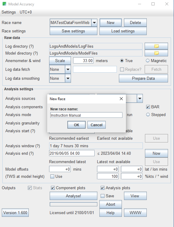 |
| Step 2 - Locate raw log files.
Model Accuracy analyzes the log files in a folder that you specify. It does not have to be where Expedition stores the files, although that folder is referenced for easy operation. You can view this quick reference by clicking on the (?) symbol to the right of the "Log Directory" label. The folder that stores the log files must contain only log files, so we recommend that you create a separate folder for the log files you want to analyze. The "subfolder" method is the recommended method of organizing log files (and is necessary any time there are log files from different sources). Model Accuracy treats each subfolder separately. The log source name is set by:
Tip: Even if you are selecting NOAA buoy data as log data to analyze, which requires fetching data from the internet, you still need to specify an empty folder where Model Accuracy can store the NOAA buoy log data |
Log Folder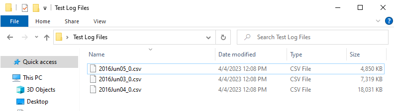 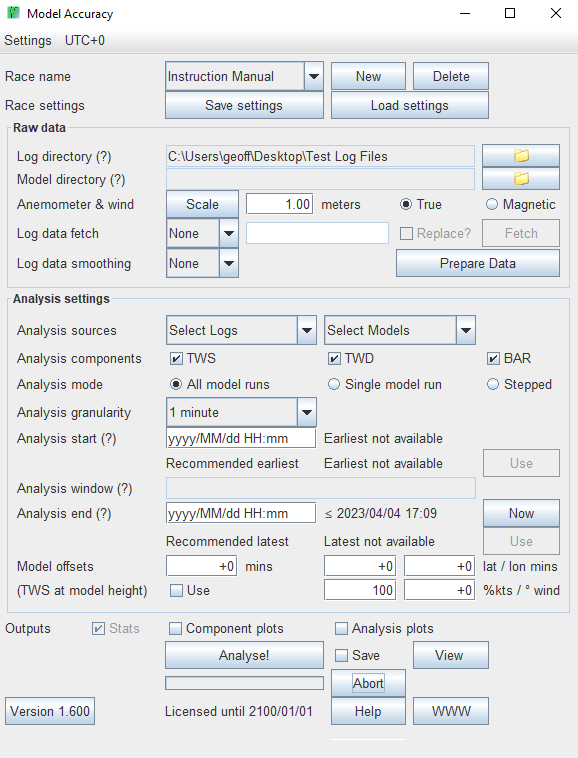 |
| Step 3 - Locate raw GRIB files.
Model Accuracy analyzes the GRIB files in a folder that you specify. It does not have to be where Expedition stores the files, although that folder is referenced for easy operation. You can view this quick reference by clicking on the (?) symbol to the right of the words "Model Directory". The folder that stores the GRIB files must contain only GRIB files, so we recommend that you create a separate folder for the GRIB files you want to analyze. The "subfolder" method is the recommended method of organizing GRIB files. Model Accuracy treats each subfolder separately. The GRIB source name is set by:
For example, if the GRIB folder has these files and folder: BIG_GRIB_1234.grbPWG_All1/PWG-42424.grb PWG_All1/BEST_PWG-64646.999.grb GFSIsNotAlwaysTheBestGRIB.grb there will then be three sources listed in the analysis: BIG_GRIB (taken from the file name)PWG_ALL1 (taken from the folder name) GFS (GFS is well known) | GRIB Folder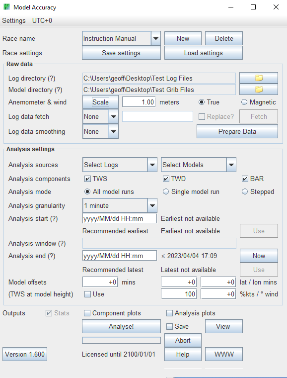 |
| Step 4 - Anemometer Setup.
Set mast height. This is the distance in meters from the water line to the anemometer where the logged wind data is captured. Scale/Report Button: True or Magnetic Degrees: |
Scale Button Report Button:  |
| Step 5 -
Put your log and GRIB files in the raw directories.
In this latest version of Model Accuracy you no longer have to select what type of log file format you are using in your analysis. Model Accuracy can now automatically detect the type of log file for Expedition, Adrena, NMEA, NOAA, AuBOM, and PredictWind file formats. | |
|
Step 5 - Adrena English version Save the log files with a .adrena.csv extension. Step 5 - Adrena French version Adrena (French version) saves its log files as .csv files even though the fields are really separated by a semi-colon. Change the file extension to .adrena.txt. |
Adrena (French version) Log file folder:  Adrena (French version) Log file folder: Step 2 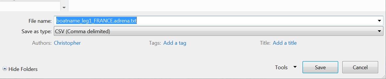 Adrena (French version) Log file folder: Step 3 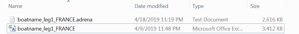 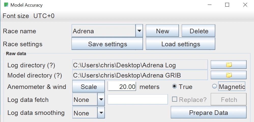 |
| Step 5 - AuBOM AuBOM (Australian Bureau of Meterorology) weather observation stations have TWS and TWD data that is capable of being downloaded similar to American NOAA weather buoys. However, the AuBOM weather observations have to be manually downloaded from each individual weather station's website. We hope to automate this soon! The file format of the AuBOM weather observations is in the .axf file format. Model Accuracy will automatically convert the .axf file format into the .csv file format required for analysis. As the user, you simply have to download the weather observation station .axf file and store on your computer in a log folder. How to download an AuBOM weather observation stations log file:
|
AuBOM Log file download process: Step 1: Note height of observation station's anemometer - enter into Model Accuracy. 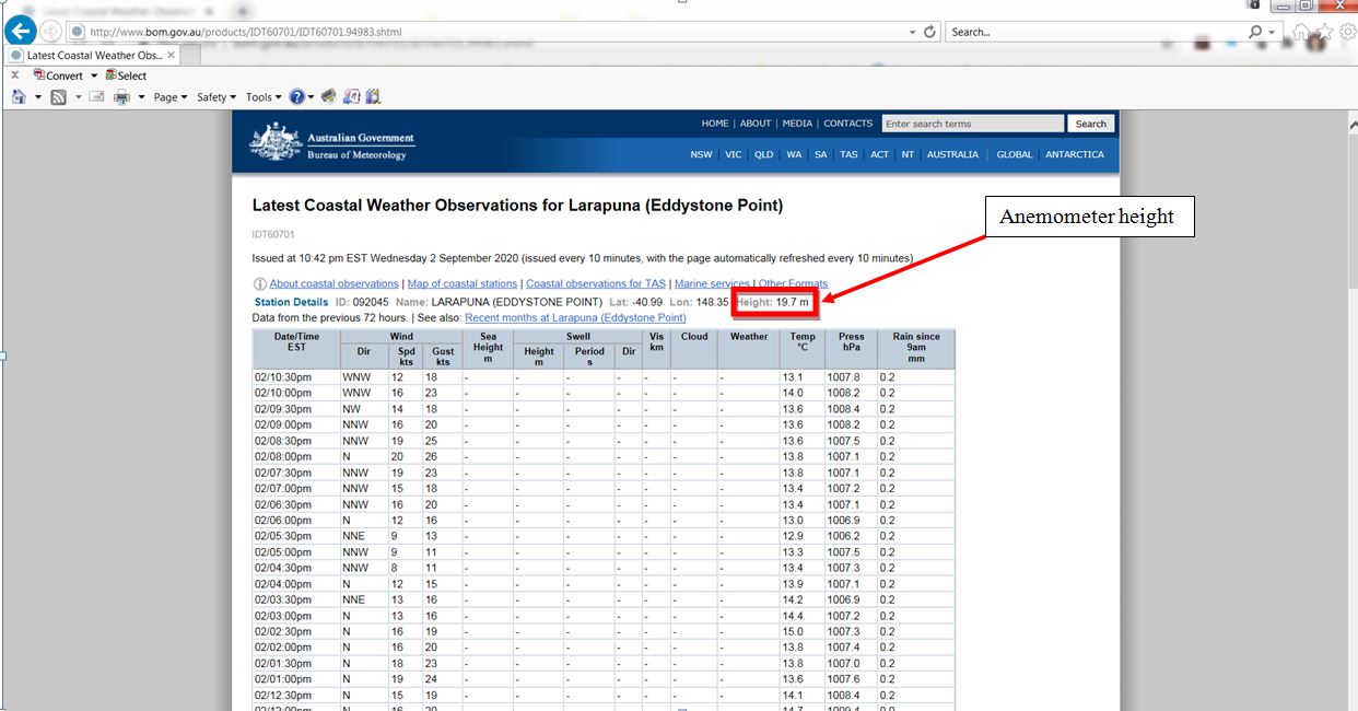 Step 2: Scroll to the bottom and download observation station's log file 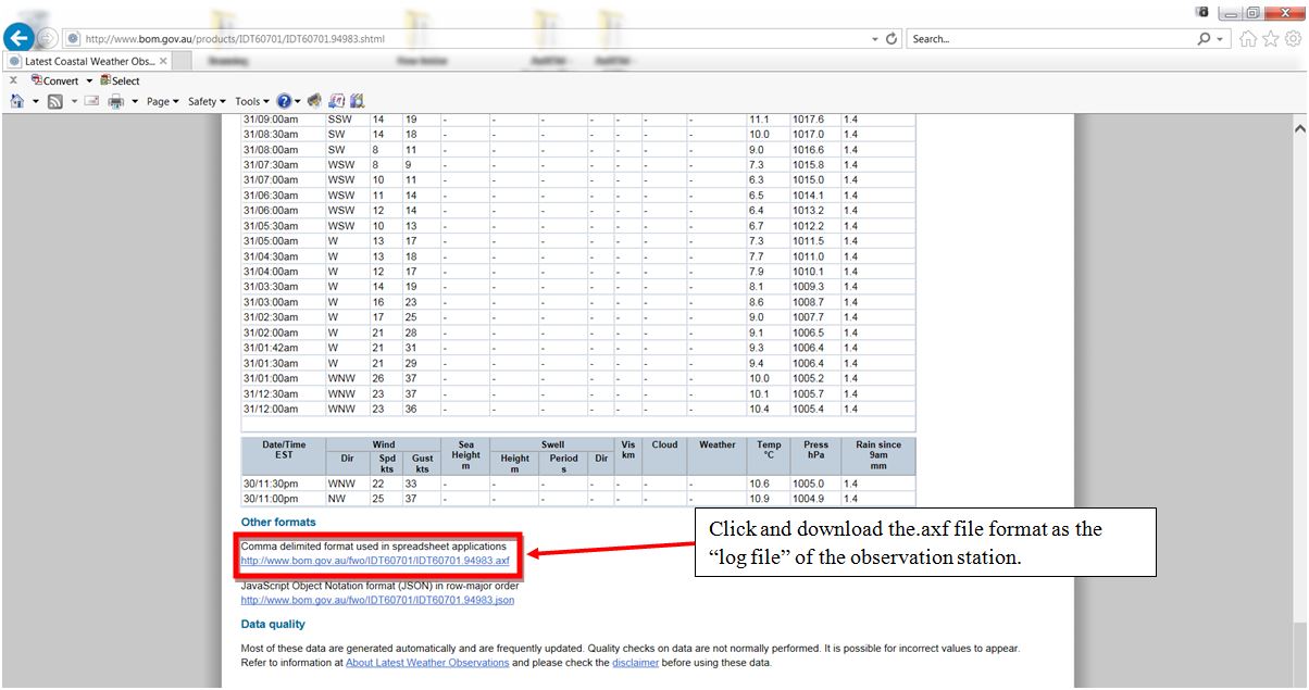 |
|
Step 5 - NMEA The file must have a .nmea.txt file extension. Your NMEA log file format should look like this format in the raw log file folder. |
NMEA Log file folder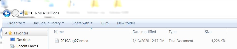 |
| Step 5 - NOAA Buoy If selecting a NOAA buoy log file you must enter the 5 digit code associated with the buoy, and select "Fetch" to the right of the code entry space. All NOAA buoy codes are listed here: https://www.ndbc.noaa.gov. NOAA buoy data is only available for the past 45 days from when selected. Example buoy code: PVGF1 is Port Everglades. Not all NOAA buoys have TWS and TWD data, so make sure to confirm yourself on the website of that particular buoy before selection. |
NOAA Buoy setup |
| Step 6 - Prepare data.
Set boat data smoothing window. This smooths out the boat log data, removing large changes in short time period that are caused by, e.g., the swinging of the mast, short gusts of wind, etc. Prepare Data - This feature prepares the log and GRIB data. It determines the earliest and recommended analysis start times, and the latest and recommended analysis end times. Model Accuracy recommends using the Prepare Data capability before every analysis! |
Smoothing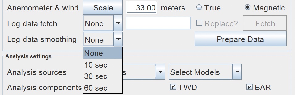 Prepare Data 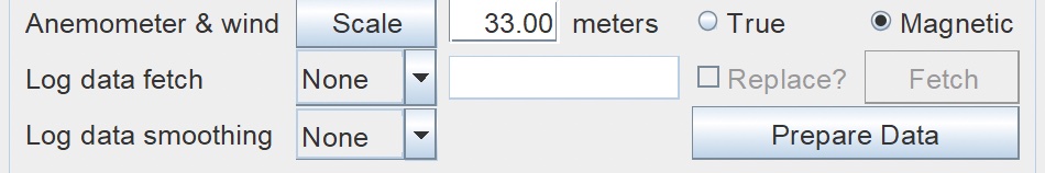 |
| Step 7 - Select the analysis sources.
Model Accuracy permits you to prepare data for and then select more than one log file and more than one GRIB model at a time. Here you can select which log files and GRIB models you are going to analyze. Most analyses are complete by selecting "All". If you would like to focus in your analysis on specific logs or GRIBs you have that option in these drop down menus. |
Select Logs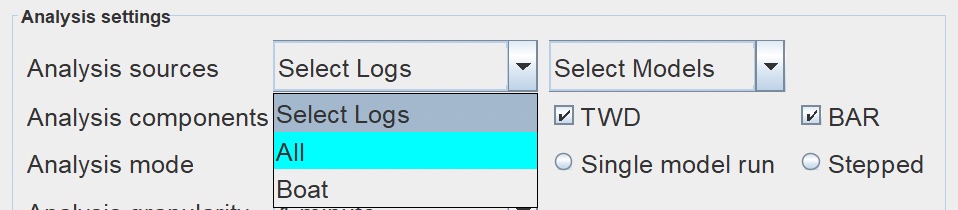 Select Models 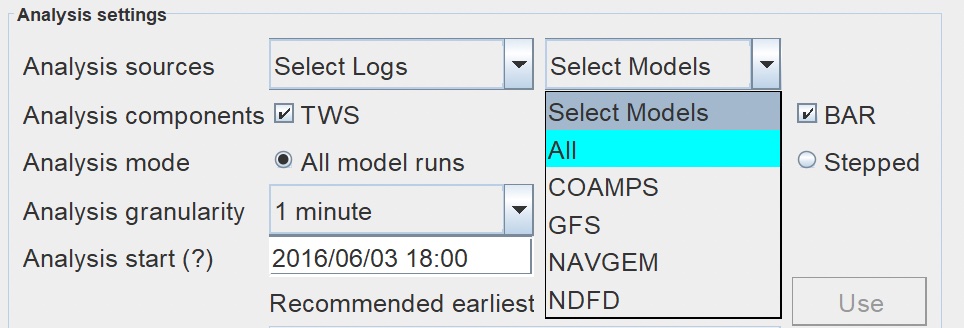 |
| Step 8 - Select analysis mode.
"All GRIB runs" creates an analysis on the freshest available data within the GRIB folder, reviewing all the GRIB files available. "Single GRIB run" allows you to analyze only one GRIB file to compare against the boat log files. Model Accuracy will choose the GRIB file with a start time closest to the start time of the analysis window you select. "Stepped" allows you to select time steps of 6, 12, 24, 48 hours within each GRIB file source to review its accuracy. This is helpful in determining the trends of each GRIB file for comparison. |
Select Analysis Mode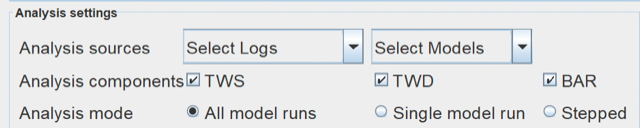 |
| Step 9 - Set analysis start and end times.
Here you tell Model Accuracy exactly from when to when you want the boat log files compared to the GRIB files. The times must be within the range of the boat log files' data and the GRIB files' data. Example: If you have Logs which cover Friday and Saturday, and GRIBs which cover Saturday and Sunday, Model Accuracy can only provide you an analysis of what took place on Saturday as that is the only time that has logs and GRIBs. By clicking the Prepare Data button earlier in the set up process Model Accuracy is capable of determining the earliest start and latest times possible for analysis, and will provide you a "no earlier than" and a "no later than" recommendation. These time recommendations are the earliest and latest time where both GRIBs and boat logs overlap. The "Use" buttons to the right of the recommended times allow the user to immediately accept the recommendations of the start/end time and use at as the analysis start/end time. Consult the Model Accuracy Manual "Warnings - Notes - Definitions" which is located at the bottom of this document for more information regarding the meaning of the recommended times. Set analysis granularity. Model Accuracy can produce results accurate to the minute, but if that's too slow for a very long log you change the granularity to take larger steps through the log data. |
Start and End Times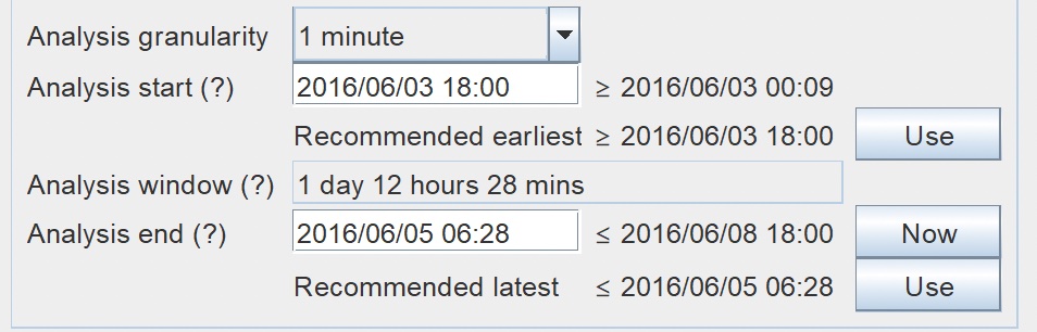 |
| Step 10 - Set offsets.
Here you can move the GRIB model in time and space, and provide offsets for the TWS and TWD.
Providing offsets for the time/latitude/longitude can be thought of as fixing possible causes for the errors in the model's prediction of TWS and TWD. Typically either only one of the sets would be used: TWS and TWD offsets, or time/latitude/longitude offsets. Select the "Use" button to apply the offsets during analysis. |
Offsets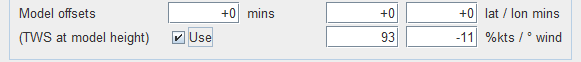 |
| Step 11 - Select results.
Select "Component Plots" if you would like to see the TWS, TWD and BAR graphical plots in addition to the statistical analysis provided. Select "Analysis Plots" if you would like to see the TWS, TWD and Model Accuracy % graphical plots in addition to the statistical analysis provided. Select "Save" to save your results and data plots for future reference, in the SavedAnalyses subfolder of the race folder created in Step 1. You must click "Save" before you click "Analyse". After analysis you can select "View" to see the saved analysis and plots of your data. |
Results Options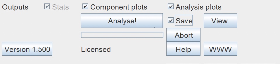 |
| Step 11 - Click "Analyse!" |
How to Understand the Analysis
Model Accuracy Results Page: Provides the statistical analysis, trend errors, and overall GRIB file recommendation.
  ----------------------------------------------------------------------------
  Analysis for MATestDataFromWeb
  Log data source is Boat
  ALL_MODELS mode
  Analysis start: 2016/06/03 23:00 UTC+0  Analysis end: 2016/06/05 06:00 UTC+0  Granularity: 00:01:00

  COAMPS: Earliest step used:
  COAMPS_20160603_1200_0009.grib    Updates 03:00 to 03:00 hh:mm apart. GRIB data point resolution 7.8 to 59.7 nm apart.
      TWS: Trend correlation  52%, RMS error   2.4, Average error   0.3 knots   above    log data. Calibrate  -0.3 knots ( 95%)
      TWD: Trend correlation  53%, RMS error  43.9, Average error   2.3 degrees right of log data. Calibrate  -2.3 degrees
      MA accuracy for Boat:COAMPS = 67% (1861 data points)

  GFS: Earliest step used:
  GFS_20160603_1800_0003.grib    Updates 03:00 to 03:00 hh:mm apart. GRIB data point resolution 13.0 to 60.1 nm apart.
      TWS: Trend correlation  38%, RMS error   4.4, Average error   1.8 knots   below    log data. Calibrate  +1.8 knots (133%)
      TWD: Trend correlation -39%, RMS error  67.9, Average error   0.4 degrees left of  log data. Calibrate  +0.4 degrees
      MA accuracy for Boat:GFS = 47% (1861 data points)

  NAVGEM: Earliest step used:
  NAVGEM_20160603_1200_0009.grib    Updates 03:00 to 03:00 hh:mm apart. GRIB data point resolution 26.5 to 60.1 nm apart.
      TWS: Trend correlation  55%, RMS error   2.4, Average error   0.8 knots   below    log data. Calibrate  +0.8 knots (112%)
      TWD: Trend correlation  10%, RMS error  63.8, Average error   9.7 degrees right of log data. Calibrate  -9.7 degrees
      MA accuracy for Boat:NAVGEM = 59% (1861 data points)

  NDFD: Earliest step used:
  NDFD_20160603_1800_0003.grib    Updates 03:00 to 03:00 hh:mm apart. GRIB data point resolution 26.0 to 30.1 nm apart.
      TWS: Trend correlation  61%, RMS error   2.5, Average error   0.9 knots   below    log data. Calibrate  +0.9 knots (114%)
      TWD: Trend correlation  12%, RMS error  58.0, Average error  20.7 degrees right of log data. Calibrate -20.7 degrees
      MA accuracy for Boat:NDFD = 61% (1861 data points)

  Model Accuracy recommends COAMPS. MA accuracy for Boat:COAMPS = 67% (1861 data points)
  ----------------------------------------------------------------------------

  ----------------------------------------------------------------------------
  Analysis settings:
      MA version                     1.600
      Race name                      MATestDataFromWeb
      Log data sources               [Boat]
      Model sources                  [COAMPS, GFS, NAVGEM, NDFD]
      Raw log directory              LogsAndModels/LogFiles
      Raw model directory            LogsAndModels/ModelFiles
      Wind height scaling            Scale
      Wind direction type            True
      Anemometer height              33.0m
      Data smoothing window          0s
      Logs analysed                  [Boat]
      Models analysed                All
      Analysis mode                  ALL_MODELS
      Analysis start time            2016/06/03 23:00 UTC+0
      Analysis window size           31:00 hh:mm
      Analysis end time              2016/06/05 06:00 UTC+0
      Analysis granularity           60s
      Offsets                        Time     0min, LAT    0min, LON    0min, TWS 100%kts, TWD   +0°
  ----------------------------------------------------------------------------
- Trend correlation: High is good!
Tells you if the GRIB prediction followed the boat log data in parallel. Example: If the TWS was predicted to increase and the boat data did in fact increase the correlation will be high. - RMS Error: LOW is good!
This is the most accurate error measure, taking into account how much time the prediction spent not aligning with the boat data ("aboves" and "belows" do not cancel each other out!). - Average Error: LOW is good!
This is the simple comparison if you averaged all the differences between the GRIB data and the boat log data. In theory here you can have a GRIB prediction way above and then way below but then averages to the exact average number of the boat data and have a zero average error, i.e.,"aboves" and "belows" do cancel each other out.- Calibrate: Use in Expedition!
Provides the simple calibration for optimal routing. For example, if the average error of the TWS forecast was 1.4 knots below log data then the recommendation would be to "Calibrate +1.4 knots" meaning that increasing TWS that amount would achieve 100% accuracy. Model Accuracy also offers a TWS % calibration value to provide the same format that Expedition accepts when adjusting TWS values in a weather forecast, e.g., 93% means you have to increase the TWS by 28% to achieve 100% accuracy. Expedition accepts 100% as the starting point for any TWS % value, and the reported value in Model Accuracy can be copied across directly. - Calibrate: Use in Expedition!
True Wind Speed Graphical Plot: Allows the user to visually track the forecasted accuracy of each GRIB vs. the logged TWS captured by the instruments onboard. Each GRIB is color coded and the black line is the boat's TWS plot.
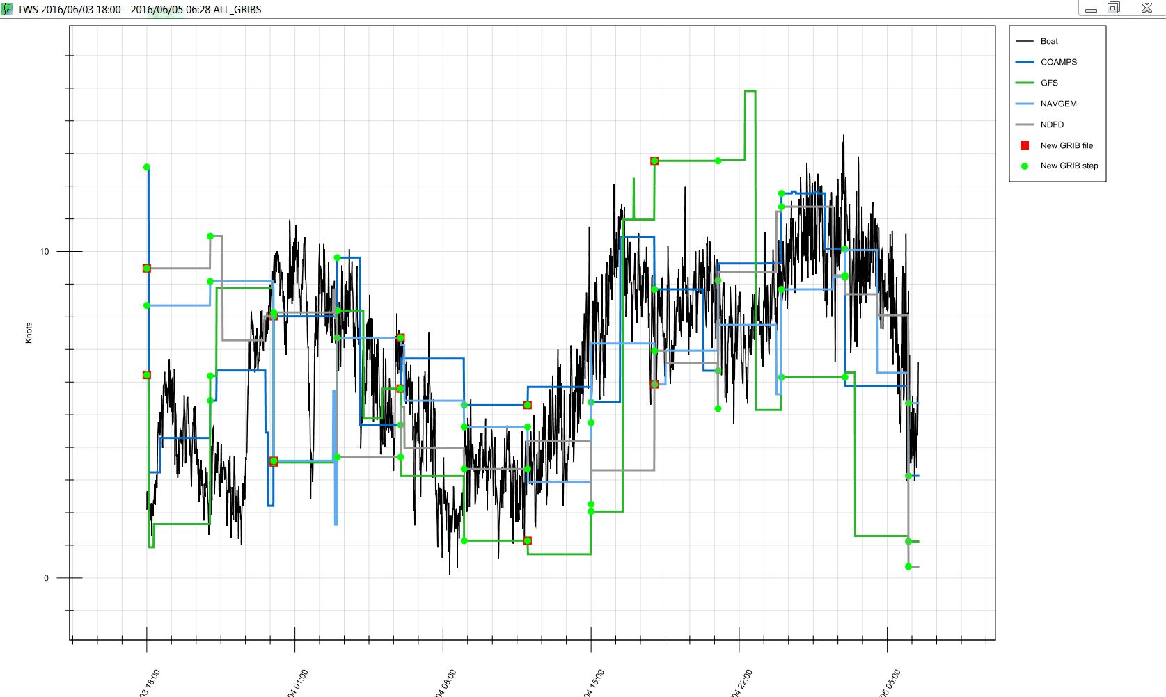
- Red Squares: represent GRIB delivery times (when you got a new GRIB). This is most commonly every 6hrs or 12hrs.
-
Green Circles: represent each "time step"
inside the respective GRIB file. Example: 3hr steps within the forecast.
True Wind Direction Graphical Plot: Displayed as a rolling figure within the chart plot. The data can "roll" from 000 degrees to 359 degrees, and the plot wraps around.
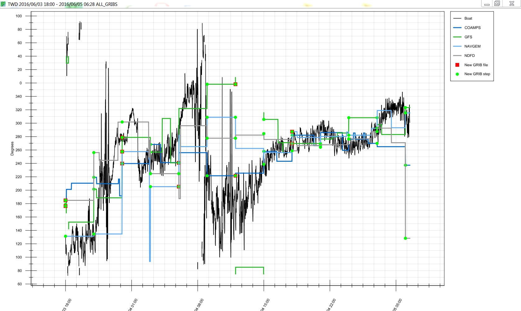
- Red Squares: represent GRIB delivery times (when you got a new GRIB). This is most commonly every 6hrs or 12hrs.
- Green Circles: represent each "time step" inside the respective GRIB file. Example: 3hr steps within the forecast.
Barometric Pressure Graphical Plot: Displayed values in millibars of pressure. Helpful to understand overall accuracy of large weather systems.
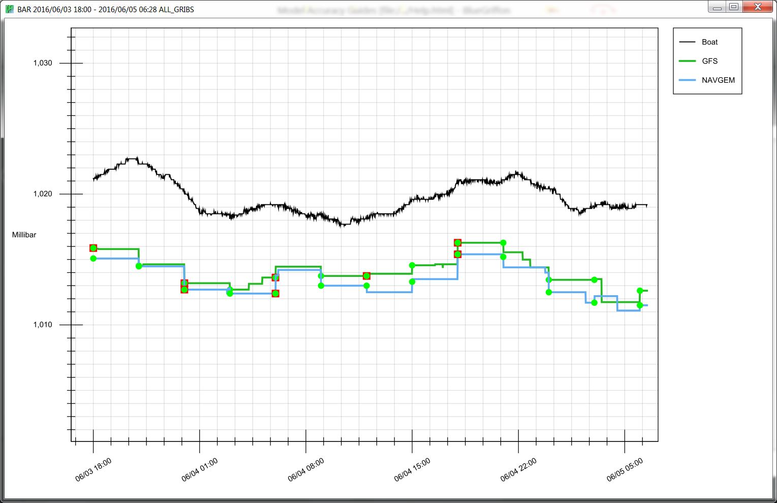
- Red Squares: represent GRIB delivery times (when you got a new GRIB). This is most commonly every 6hrs or 12hrs.
- Green Circles: represent each "time step" inside the respective GRIB file. Example: 3hr steps within the forecast.
True Wind Direction Error Graphical Plot: Displayed as degrees of error per GRIB file left or right of the boat's instrument data plotted in time. The closer the plot is to a straight line the less TWD error of that particular GRIB.
- Red Squares: represent GRIB delivery times (when you got a new GRIB). This is most commonly every 6hrs or 12hrs.
- Green Circles: represent each "time step" inside the respective GRIB file. Example: 3hr steps within the forecast.
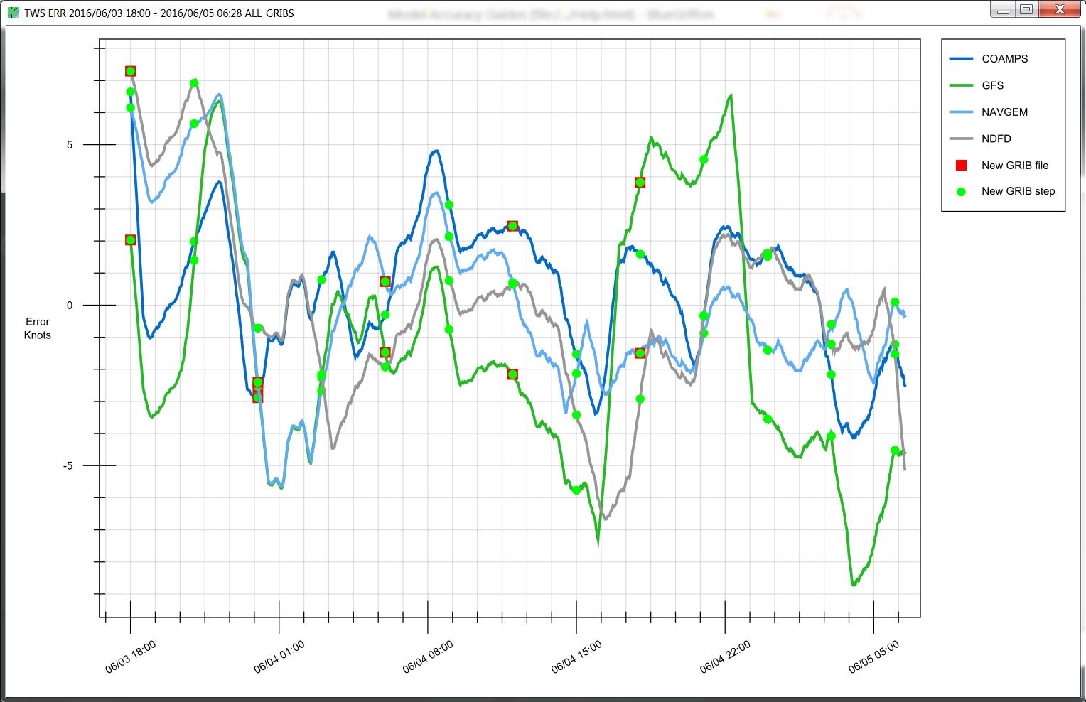
True Wind Speed Error Graphical Plot: Displayed as knots of error per GRIB file above or below of the boat's instrument data plotted in time. The closer the plot is to a straight line the less TWS error of that particular GRIB.
- Red Squares: represent GRIB delivery times (when you got a new GRIB). This is most commonly every 6hrs or 12hrs.
- Green Circles: represent each "time step" inside the respective GRIB file. Example: 3hr steps within the forecast.
Model Accuracy % Graphical Plot: Displayed as values 0-100% of accuracy per GRIB file plotted in time. The closer the line is to 100% the more accurate that respective GRIB file. Helps understand exactly when the accuracy of a GRIB file was best or worst and which GRIB file source performed the best in what conditions.
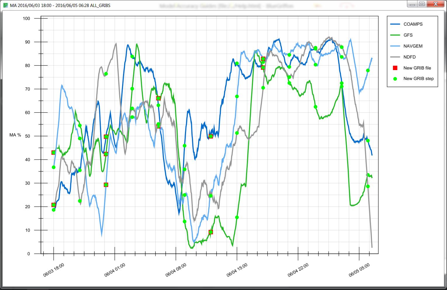
- Red Squares: represent GRIB delivery times (when you got a new GRIB). This is most commonly every 6hrs or 12hrs.
- Green Circles: represent each "time step" inside the respective GRIB file. Example: 3hr steps within the forecast.
Analysis Mode Definitions
All GRIB runs Analysis mode: Compares the freshest GRIB data to the boat log data. For example, if you get a new GRIB every 6 hours then the oldest GRIB data that will be analyzed in this mode is 6 hours old. This is a broad and general analysis to determine which GRIB is doing well at predicting weather. (most common analysis)Single GRIB Analysis mode: Compares a single chosen GRIB file (one source, one delivery time) to the boat log data.
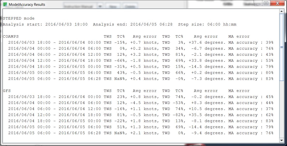
Stepped Analysis mode: Compares a chosen GRIB delivery time of all the GRIBs in the folder, by examining in small blocks of time within the analysis time frame set by the user. The user can choose the size of the blocks of time to compare within the overall analysis (6 hr, 12 hr, 24 hr, 48 hr). This mode is helpful to see the trend more clearly of when each GRIB's forecast gets inaccurate. The stepped mode outputs the results in blocks of times analyzed. Example:
Warnings and Notes
- Your computer must be set to Zulu time or the appropriate time zone for your location. This allows the boat log file to be time-stamped in the same way that the GRIB files are created (i.e., in Zulu time).
- Model Accuracy applies the appropriate variation as applicable to the GRIB files. Make sure you understand how your TWD is being stored in your GRIB files as either True or Magnetic. Consult your settings in Expedition to make sure you select the proper setting in Model Accuracy.
- The height of your anemometer (wind instruments on your mast) must be entered in meters. This measurement is from the waterline to the anemometer (birdie and cups).
- Model Accuracy will read only .grb and .grb2 type GRIB files.
- The time selected for the analysis must be covered by both the boat log files and GRIB files, or else the analysis will not work. Use the Advanced Data Preparation button/feature to help learn what are the earliest and latest times where both the GRIB and log files overlap in your folder.
- Analysis Start Times: The EARLIEST start time is constrained by the start of the boat log data & the single earliest GRIB run. If you start the analysis at this time only that one GRIB source gets analyzed (because the others start later). The RECOMMENDED earliest start time is constrained by the start of the boat log data and the latest GRIB run. If you start the analysis at this time all GRIB sources get analyzed.
- Analysis End Times: The LATEST end time is constrained by the end of the boat log data and the single latest GRIB step time. If you end the analysis at this time only that GRIB has data (in the form of a GRIB step) at the end time. The others will have older data (because their last GRIB steps are earlier). The recommended latest end time is constrained by the end of the boat log data and the earliest last GRIB step time. If you end the analysis at this time all the GRIBs have data (in the form of a GRIB step) at the end time.
- It is recommended that you keep all of your GRIB files organized by Zulu run time in separate folders, as you download them. When you run an analysis, create a new folder of all the GRIBs you want to analyze and specify that folder as outlined in Step 3 of the instruction manual.
- It is recommended that you rename each GRIB file that you download.
This is can be tedious, however it helps you quickly identify each
individual GRIB file for future analysis, and ensures as a navigator you
always know which GRIB you are using. For example:
